Virtual Cameras and Spatial Transformations
Defining a Space: We define a space with a point of origin and a set of axes. A single point in space can be represented as infinitely many different coordinates just by changing the coordinate system.
Rasterizing 3D Scenes
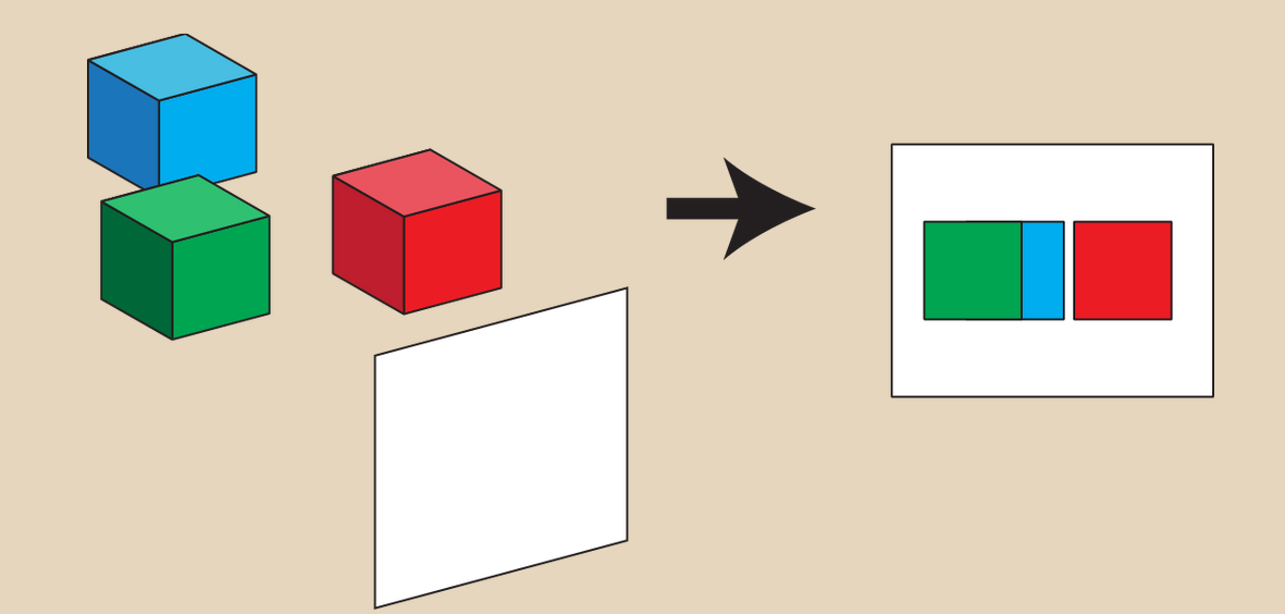
So far, we have been rasterizing 2D scenes with 2D geometry. This is easy, as the 2D shapes are already what they are in our viewing plane. However, 3D geometry data must somehow be projected down to a 2D space so it can be visible on our 2D screen.
One simple solution is to ignore the Z coordinate. This gives us what we call orthographic projection.
Orthographic projection is fine for some applications. However, it is not ideal. We want to simulate what the eye sees. Our eye works as a point rather than a plane. This allows us to see depth. Currently, because we ignore the Z coordinate, objects look the same no matter how far they are from the screen. Instead, we want to use perspective projection. We want to simulate what is called a pinhole camera.
Pinhole Camera
In a pinhole camera, light from the world passes through a tiny hole onto some sensor. The sensor interprets the light as color and produces an image. Generally, this is the type of camera that we simulate in computer graphics.
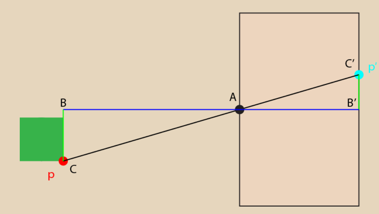
Given a world point $p$ here and its projected point $p$ in the camera, we see that $p’$ will scale based on $p’s$ distance from A. We can create a pair of similar triangles, and then write a relationship between the y-coordinate of $p$ and the y-coordinate of $p’$. $$ p’_y = \frac{p_y \cdot p’_z }{p_z} $$ This technique is known as perspective-divide. It also applies to the x-coordinate.
After we apply perspective-divide, the geometry is still 3D, just deformed to account for the perspective diminishing of the geometry. However, it will now look far more accurate through the orthographic projection we threw earlier.
Field of View
In a physical pinhole camera, the focal length determines the field of view. This is the distance between the pinhole and the display screen. In the case of the above image, the distance $A \to B’$ would be the focal length. The less the focal length(the closer the screen is to the pinhole), the more of the world it can see. And since you’re fitting more of the world onto a equivalently sized screen, everything will look a little smaller.
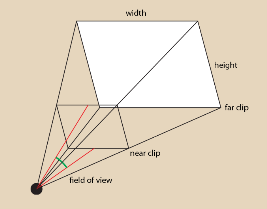
Perspective Frustum
We can visualize the volume in which objects are visible to our camera. The bounds are created by three components:
- Field of view
- Aspect ratio: screen width over height
- Near clip and far clip planes
- Two planes that clip the depth of objects visible by the camera
- They allow us to make sure we are not drawing too many things, and allows us to quantify the distance of an object from the camera as a normalized value
Projection Matrix
Now that we have the entire projection process, we want to mathematically represent our camera frustum. We want to project our perspective camera coordinates into screen space coordinates. This will determine what geometry is within our frustum bounds. We could perform all these operations as hand coded transformations, but its much easier to create a single matrix composed of our transformations and apply that instead.
Remember that to perform perspective divide, we want to divide the x and y coordinates by the z coordinate. But how can we do that if we have already multiplied the matrix by our point?
Remember that when we use homogenous coordinates, we always divide our vector by $W$ to make sure that we keep the homogenous coordinate 1 and stay in cartesian coordinates. This ends up helping us, as we can just set $W$ to the z coordinate, which will result in all the coordinates being divided by $z$ to achieve correct vectors. The matrix looks like this: $$ \begin{bmatrix} 1 & 0 & 0 & 0 \newline 0 & 1 & 0 & 0 \newline 0 & 0 & 1 & 0 \newline 0 & 0 & 1 & 0 \newline \end{bmatrix} $$ However, this now results in us having a Z coordinate of 1, as we are also dividing it by itself. This normalized z coordinate is useless on its own, so we need to modify our matrix to get a more useful z coordinate.
Some math has already been done to account for all this. The final matrix looks like such: $$ \begin{bmatrix} 1 & 0 & 0 & 0 \newline 0 & 1 & 0 & 0 \newline 0 & 0 & P & Q \newline 0 & 0 & 1 & 0 \newline \end{bmatrix} $$
- $P = \frac{f}{f-n}$
- $Q = \frac{-fn}{f-n}$
- $f$ is the far clip distance
- $n$ is the near clip distance
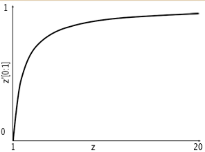
This matrix will map $z$ to a range [0, 1] where either end sits at a clipping plane distance. If you do the calculations yourself, when $z = n$, you’ll see $z’ = 0$, and when $z=f$, then $z’ = 1$.
Note that the change in value of $z’$ between the near clip and far clip planes is not linear. The computation involves division by $W’$, so the curve looks like this:
If the near and far clip planes are too far apart, you can also get some z-fighting due to floating point errors.
Fitting to a Screen
Now that we have performed perspective divide, we need to map the data to our screen. For this, we need to get normalized screen coordinates, and determine the range of XY coordinates we will map to our screen. The convention is to declare the lower-left corner of the screen as $[-1, -1]$ and the upper right corner as $[1, 1$] regardless of aspect ratio.
As stated before, as the FOV of the virtual camera increases, we should see more of the world. Therefore, the scale of the scene’s geometry is inversely proportional to the camera’s FOV. We can use trigonometry to get the relationship we need between FOV and scale.
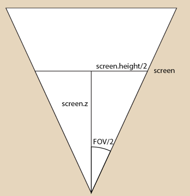
$$ tan(\frac{FOV}{2}) = (\frac{screen.height}{2})/screen.z $$ If we assume the screen is always 1 unit away, we get $tan(\frac{FOV}{2}) = (\frac{screen.height}{2})$. However, right now, it looks like our screen is scaling with the FOV of our camera. We want our screen to remain the same size. To do this, we will scale our geometry by the inverse of the tangent:
$$ \begin{bmatrix} \frac{S}{A} & 0 & 0 & 0 \newline 0 & S & 0 & 0 \newline 0 & 0 & P & Q \newline 0 & 0 & 1 & 0 \end{bmatrix} $$
- $P = \frac{f}{f-n}$
- $Q = \frac{-fn}{f-n}$
- $S = \frac{1}{tan(FOV/2)}$
- $A = \frac{width}{height}$
Projection Matrix Summary
- Scale W by Z to perform perspective divide
- Scale Z to [0, 1] range(normalize) between the clipping planes
- Scale XY to [-1, 1] range based on FOV and aspect ratio
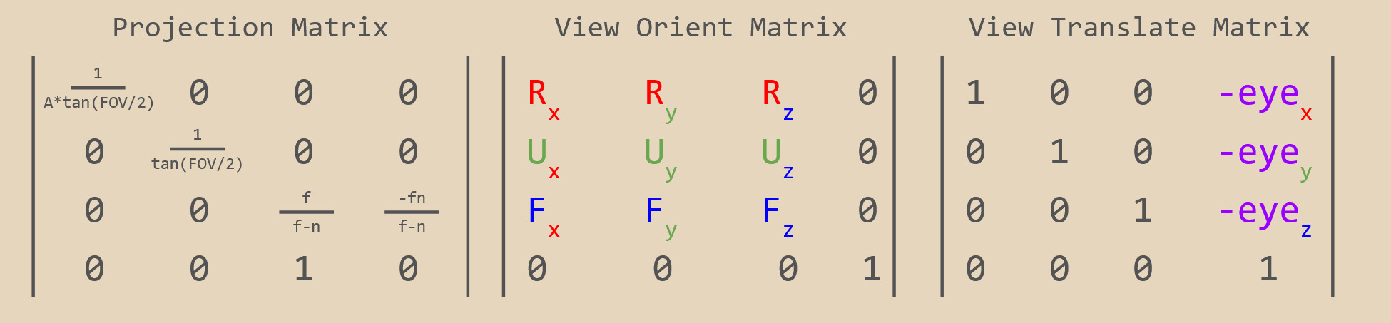
$$ \begin{bmatrix} \frac{1}{A*tan(FOV/2)} & 0 & 0 & 0 \newline 0 & \frac{1}{tan(FOV/2)} & 0 & 0 \newline 0 & 0 & \frac{f}{f-n} & \frac{-fn}{f-n} \newline 0 & 0 & 1 & 0 \end{bmatrix} $$
View Matrix
All the computations we have performed so far have assumed geometry position is framed relative to the camera origin and axes. However, really, the geometry we are given is framed relative to the world origin and axes. That may not always be the case for the camera, so we need a matrix to transform us from world coordinates to camera coordinates.
View Matrix Parameters
A space coordinate system is defined by two parameters: an origin and a set of axes.
- The camera origin is simply the position the camera inhabits in the world space
- The forward direction (F), also known as the look vector, is a direction in world coordinates that represents the direction in which the camera is looking. It represents the local Z axis
- The local right (R) is a direction in world coordinates that represents the direction that is “rightward” in the camera’s local coordinates. It represents the local X axis and is perpendicular to the look direction
- The local up (U) is a direction in world coordinates that represents the direction that is “upward” in the camera’s local coordinates. It represents the local Y axis, and is perpendicular to both the local right and look direction
The view matrix transforms the geometry from world space to camera space. The camera itself is not moving; the scene’s geometry data is being transformed in the opposite way of how you want the camera to move. Strictly speaking, the “camera” does not exist. you are always transforming the geometry in your scene.
The view matrix is comprised of two sub-matrices: the orientation matrix (O) and the translation matrix (T). $$ O = \begin{bmatrix} R_x & R_y & R_z & 0 \newline U_x & U_y & U_z & 0 \newline F_x & F_y & F_z & 0 \newline 0 & 0 & 0 & 1 \end{bmatrix} $$ $$ T = \begin{bmatrix} 1 & 0 & 0 & -eye_x \newline 0 & 1 & 0 & -eye_y \newline 0 & 0 & 1 & -eye_z \newline 0 & 0 & 0 & 1 \end{bmatrix} $$ $$ ViewMatrix = O \cdot T $$ It isn’t difficult to figure out what is going on here. First you translate the geometry to be relative to the camera’s origin. Then, you perform rotations of all the geometry about the camera’s origin according to its angle.
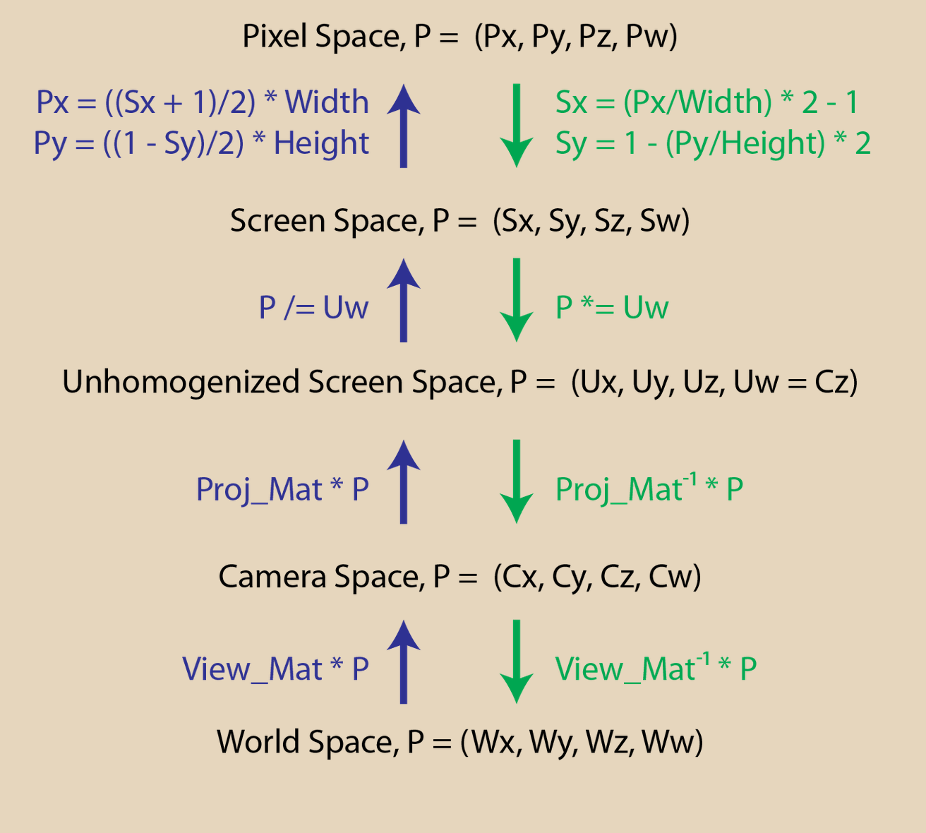
From World to Screen
We can concatenate these two matrices to see our scene. To reiterate:
- View matrix: sets up our camera’s position and orientation
- Projection matrix: Projects objects from 3D space into the screen’s 2D space, where screen space is in normalized device coordinates Note that the projection matrix is applied after the view matrix.
Converting Back to Pixel Coordinates
Finally, the matrices we have so far will convert our geometry from world space to normalized pixel coordinates. We want our geometry in regular old pixel coordinates. Therefore, we just need to multiply by our aspect ratio: $$ Pixel.x = (NDC.x + 1) * \frac{width}{2} $$ $$ Pixel.y = (1-NDC.y) * \frac{height}{2} $$
Summary
In summary, here are the camera transformations: